Stock Analysis and Data Visualization
Follow along: Stock Analysis and Data Visualization
- Create a new *.ipynb file Jupyter Notebook
- Fill in the content below in the newly created file
- Follow and Execute the example codes
Object
To analyze stock prices, ‘fundamental analysis’ and ‘technical analysis’ are typically used.
‘Fundamental analysis’ is a method of evaluating and analyzing the intrinsic value of stocks by examining various financial and economic factors of a company.
‘Technical analysis’ is a method of predicting stock price movements by using various technical indicators such as trend lines, patterns, moving averages, and relative strength index (RSI) on company stock price charts and trading volume.
Using code, the company’s past stock price data is retrieved, analyzed using representative technical indicators, and visualized and displayed.
Data Analysis
ferrari_quote.csv

tesla_quote.csv

Attributes of file
Date: Stock market opening date
Open: Stock price (market price) at the start of the market
High: Highest price during the session (high price)
Low: lowest price during the session (low price)
Close: Price at market close (closing price)
Adj Close: Modified closing price considering ex-dividends, etc.
Volume: stock trading volume
Candlestick Chart Visualization
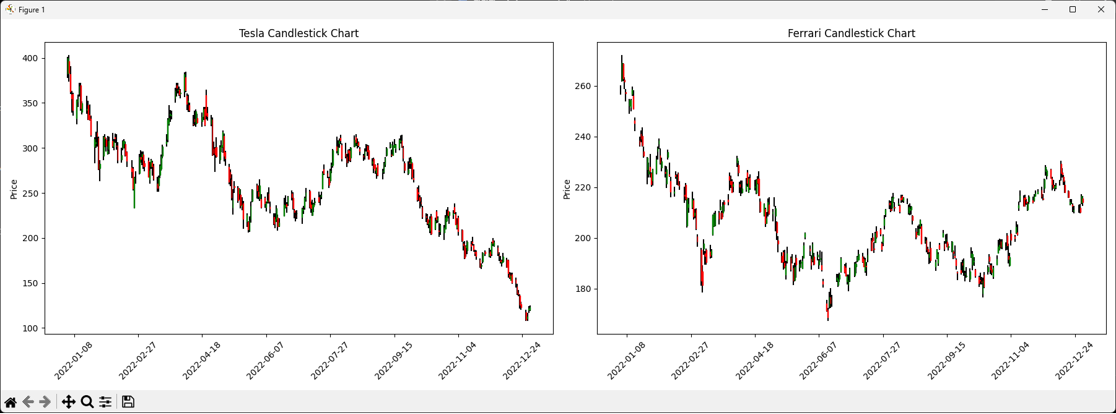
Draw a candle chart using the opening price, high price, low price, and closing price from 2022-01-01 to 2022-12-31.
1.chart.py
import pandas as pd
import matplotlib.pyplot as plt
import matplotlib.dates as mdates

# Load Tesla and Ferrari stock data
tesla_data = pd.read_csv('tesla_quote.csv', parse_dates=True, index_col='Date')
ferrari_data = pd.read_csv('ferrari_quote.csv', parse_dates=True, index_col='Date')

# Define the period for both charts (e.g., '2022-01-01' to '2022-12-31')
start_date = '2022-01-01'
end_date = '2022-12-31'

# Filter dataframes to include only the specified period
tesla_data = tesla_data[(tesla_data.index >= start_date) & (tesla_data.index <= end_date)]
ferrari_data = ferrari_data[(ferrari_data.index >= start_date) & (ferrari_data.index <= end_date)]

# Create subplots with 2 columns to display charts side by side
fig, (ax1, ax2) = plt.subplots(nrows=1, ncols=2, figsize=(18, 6))

# Define candlestick colors
up_color = 'g'
down_color = 'r'

# Plot Tesla candlesticks
for idx, row in tesla_data.iterrows():
    open_price = row['Open']
    close_price = row['Close']
    high_price = row['High']
    low_price = row['Low']

    if close_price > open_price:
        color = up_color
        rect_height = close_price - open_price
        y = open_price
    else:
        color = down_color
        rect_height = open_price - close_price
        y = close_price

    ax1.add_patch(plt.Rectangle((mdates.date2num(idx) - 0.2, y), 0.4, rect_height, fill=True, color=color, zorder=2))
    ax1.plot([mdates.date2num(idx), mdates.date2num(idx)], [low_price, high_price], color='black', zorder=1)

# Set x-axis format for Tesla chart
ax1.xaxis.set_major_formatter(mdates.DateFormatter("%Y-%m-%d"))
ax1.set_ylabel('Price')
ax1.set_title('Tesla Candlestick Chart')
ax1.tick_params(axis='x', rotation=45)

# Plot Ferrari candlesticks
for idx, row in ferrari_data.iterrows():
    open_price = row['Open']
    close_price = row['Close']
    high_price = row['High']
    low_price = row['Low']

    if close_price > open_price:
        color = up_color
        rect_height = close_price - open_price
        y = open_price
    else:
        color = down_color
        rect_height = open_price - close_price
        y = close_price

    ax2.add_patch(plt.Rectangle((mdates.date2num(idx) - 0.2, y), 0.4, rect_height, fill=True, color=color, zorder=2))
    ax2.plot([mdates.date2num(idx), mdates.date2num(idx)], [low_price, high_price], color='black', zorder=1)

# Set x-axis format for Ferrari chart
ax2.xaxis.set_major_formatter(mdates.DateFormatter("%Y-%m-%d"))
ax2.set_ylabel('Price')
ax2.set_title('Ferrari Candlestick Chart')
ax2.tick_params(axis='x', rotation=45)

# Adjust layout and show both charts
plt.tight_layout()
plt.show()
Closing Price 20-day Moving Average Visualization
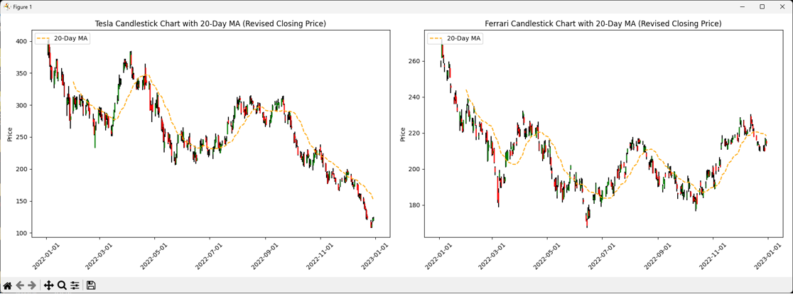
Draw a 20-day moving average based on the closing price.
2.20ma.py
import pandas as pd
import matplotlib.pyplot as plt
import matplotlib.dates as mdates

# Load Tesla and Ferrari stock data
tesla_data = pd.read_csv('tesla_quote.csv', parse_dates=True, index_col='Date')
ferrari_data = pd.read_csv('ferrari_quote.csv', parse_dates=True, index_col='Date')

# Define the period for both charts (e.g., '2022-01-01' to '2022-12-31')
start_date = '2022-01-01'
end_date = '2022-12-31'

# Filter dataframes to include only the specified period
tesla_data = tesla_data[(tesla_data.index >= start_date) & (tesla_data.index <= end_date)]
ferrari_data = ferrari_data[(ferrari_data.index >= start_date) & (ferrari_data.index <= end_date)]

# Create subplots with 2 columns to display charts side by side
fig, (ax1, ax2) = plt.subplots(nrows=1, ncols=2, figsize=(18, 6))

# Define candlestick colors
up_color = 'g'
down_color = 'r'

# Plot Tesla candlesticks and 20-day moving average
for idx, row in tesla_data.iterrows():
    open_price = row['Open']
    close_price = row['Close']
    high_price = row['High']
    low_price = row['Low']

    if close_price > open_price:
        color = up_color
        rect_height = close_price - open_price
        y = open_price
    else:
        color = down_color
        rect_height = open_price - close_price
        y = close_price

    ax1.add_patch(plt.Rectangle((mdates.date2num(idx) - 0.2, y), 0.4, rect_height, fill=True, color=color, zorder=2))
    ax1.plot([mdates.date2num(idx), mdates.date2num(idx)], [low_price, high_price], color='black', zorder=1)

# Calculate 20-day moving average for Tesla based on revised closing price
tesla_data['20D_MA'] = tesla_data['Close'].rolling(window=20).mean()
ax1.plot(tesla_data.index, tesla_data['20D_MA'], label='20-Day MA', color='orange', linestyle='--')

# Set x-axis format for Tesla chart
ax1.xaxis.set_major_formatter(mdates.DateFormatter("%Y-%m-%d"))
ax1.set_ylabel('Price')
ax1.set_title('Tesla Candlestick Chart with 20-Day MA (Revised Closing Price)')
ax1.tick_params(axis='x', rotation=45)
ax1.legend(loc='upper left')

# Plot Ferrari candlesticks and 20-day moving average
for idx, row in ferrari_data.iterrows():
    open_price = row['Open']
    close_price = row['Close']
    high_price = row['High']
    low_price = row['Low']

    if close_price > open_price:
        color = up_color
        rect_height = close_price - open_price
        y = open_price
    else:
        color = down_color
        rect_height = open_price - close_price
        y = close_price

    ax2.add_patch(plt.Rectangle((mdates.date2num(idx) - 0.2, y), 0.4, rect_height, fill=True, color=color, zorder=2))
    ax2.plot([mdates.date2num(idx), mdates.date2num(idx)], [low_price, high_price], color='black', zorder=1)

# Calculate 20-day moving average for Ferrari based on revised closing price
ferrari_data['20D_MA'] = ferrari_data['Close'].rolling(window=20).mean()
ax2.plot(ferrari_data.index, ferrari_data['20D_MA'], label='20-Day MA', color='orange', linestyle='--')

# Set x-axis format for Ferrari chart
ax2.xaxis.set_major_formatter(mdates.DateFormatter("%Y-%m-%d"))
ax2.set_ylabel('Price')
ax2.set_title('Ferrari Candlestick Chart with 20-Day MA (Revised Closing Price)')
ax2.tick_params(axis='x', rotation=45)
ax2.legend(loc='upper left')

# Adjust layout and show both charts
plt.tight_layout()
plt.show()
Closing Price 60-day Moving Average Visualization
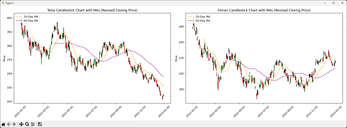
Draw a 60-day moving average based on the closing price.
3.60ma.py
import pandas as pd
import matplotlib.pyplot as plt
import matplotlib.dates as mdates

# Load Tesla and Ferrari stock data
tesla_data = pd.read_csv('tesla_quote.csv', parse_dates=True, index_col='Date')
ferrari_data = pd.read_csv('ferrari_quote.csv', parse_dates=True, index_col='Date')

# Define the period for both charts (e.g., '2022-01-01' to '2022-12-31')
start_date = '2022-01-01'
end_date = '2022-12-31'

# Filter dataframes to include only the specified period
tesla_data = tesla_data[(tesla_data.index >= start_date) & (tesla_data.index <= end_date)]
ferrari_data = ferrari_data[(ferrari_data.index >= start_date) & (ferrari_data.index <= end_date)]

# Create subplots with 2 columns to display charts side by side
fig, (ax1, ax2) = plt.subplots(nrows=1, ncols=2, figsize=(18, 6))

# Define candlestick colors
up_color = 'g'
down_color = 'r'

# Plot Tesla candlesticks and 20-day moving average
for idx, row in tesla_data.iterrows():
    open_price = row['Open']
    close_price = row['Close']
    high_price = row['High']
    low_price = row['Low']

    if close_price > open_price:
        color = up_color
        rect_height = close_price - open_price
        y = open_price
    else:
        color = down_color
        rect_height = open_price - close_price
        y = close_price

    ax1.add_patch(plt.Rectangle((mdates.date2num(idx) - 0.2, y), 0.4, rect_height, fill=True, color=color, zorder=2))
    ax1.plot([mdates.date2num(idx), mdates.date2num(idx)], [low_price, high_price], color='black', zorder=1)

# Calculate 20-day moving average for Tesla based on revised closing price
tesla_data['20D_MA'] = tesla_data['Close'].rolling(window=20).mean()
ax1.plot(tesla_data.index, tesla_data['20D_MA'], label='20-Day MA', color='orange', linestyle='--')

# Calculate 60-day moving average for Tesla based on revised closing price
tesla_data['60D_MA'] = tesla_data['Close'].rolling(window=60).mean()
ax1.plot(tesla_data.index, tesla_data['60D_MA'], label='60-Day MA', color='purple', linestyle='--')

# Set x-axis format for Tesla chart
ax1.xaxis.set_major_formatter(mdates.DateFormatter("%Y-%m-%d"))
ax1.set_ylabel('Price')
ax1.set_title('Tesla Candlestick Chart with MAs (Revised Closing Price)')
ax1.tick_params(axis='x', rotation=45)
ax1.legend(loc='upper left')

# Plot Ferrari candlesticks and 20-day moving average
for idx, row in ferrari_data.iterrows():
    open_price = row['Open']
    close_price = row['Close']
    high_price = row['High']
    low_price = row['Low']

    if close_price > open_price:
        color = up_color
        rect_height = close_price - open_price
        y = open_price
    else:
        color = down_color
        rect_height = open_price - close_price
        y = close_price

    ax2.add_patch(plt.Rectangle((mdates.date2num(idx) - 0.2, y), 0.4, rect_height, fill=True, color=color, zorder=2))
    ax2.plot([mdates.date2num(idx), mdates.date2num(idx)], [low_price, high_price], color='black', zorder=1)

# Calculate 20-day moving average for Ferrari based on revised closing price
ferrari_data['20D_MA'] = ferrari_data['Close'].rolling(window=20).mean()
ax2.plot(ferrari_data.index, ferrari_data['20D_MA'], label='20-Day MA', color='orange', linestyle='--')

# Calculate 60-day moving average for Ferrari based on revised closing price
ferrari_data['60D_MA'] = ferrari_data['Close'].rolling(window=60).mean()
ax2.plot(ferrari_data.index, ferrari_data['60D_MA'], label='60-Day MA', color='purple', linestyle='--')

# Set x-axis format for Ferrari chart
ax2.xaxis.set_major_formatter(mdates.DateFormatter("%Y-%m-%d"))
ax2.set_ylabel('Price')
ax2.set_title('Ferrari Candlestick Chart with MAs (Revised Closing Price)')
ax2.tick_params(axis='x', rotation=45)
ax2.legend(loc='upper left')

# Adjust layout and show both charts
plt.tight_layout()
plt.show()
Daily Volume Visualization
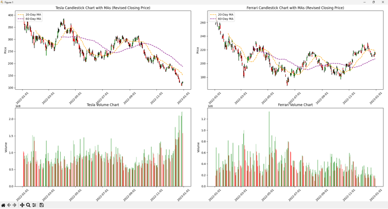
Draw a daily volume chart.
4.volume.py
import pandas as pd
import matplotlib.pyplot as plt
import matplotlib.dates as mdates

# Load Tesla and Ferrari stock data
tesla_data = pd.read_csv('tesla_quote.csv', parse_dates=True, index_col='Date')
ferrari_data = pd.read_csv('ferrari_quote.csv', parse_dates=True, index_col='Date')

# Define the period for both charts (e.g., '2022-01-01' to '2022-12-31')
start_date = '2022-01-01'
end_date = '2022-12-31'

# Filter dataframes to include only the specified period
tesla_data = tesla_data[(tesla_data.index >= start_date) & (tesla_data.index <= end_date)]
ferrari_data = ferrari_data[(ferrari_data.index >= start_date) & (ferrari_data.index <= end_date)]

# Create subplots with 2 rows and 2 columns to display charts side by side
fig, ((ax1, ax2), (ax3, ax4)) = plt.subplots(nrows=2, ncols=2, figsize=(18, 12))

# Define candlestick colors
up_color = 'g'
down_color = 'r'

# Plot Tesla candlesticks and 20-day moving average
for idx, row in tesla_data.iterrows():
    open_price = row['Open']
    close_price = row['Close']
    high_price = row['High']
    low_price = row['Low']

    if close_price > open_price:
        color = up_color
        rect_height = close_price - open_price
        y = open_price
    else:
        color = down_color
        rect_height = open_price - close_price
        y = close_price

    ax1.add_patch(plt.Rectangle((mdates.date2num(idx) - 0.2, y), 0.4, rect_height, fill=True, color=color, zorder=2))
    ax1.plot([mdates.date2num(idx), mdates.date2num(idx)], [low_price, high_price], color='black', zorder=1)

# Calculate 20-day moving average for Tesla based on revised closing price
tesla_data['20D_MA'] = tesla_data['Close'].rolling(window=20).mean()
ax1.plot(tesla_data.index, tesla_data['20D_MA'], label='20-Day MA', color='orange', linestyle='--')

# Calculate 60-day moving average for Tesla based on revised closing price
tesla_data['60D_MA'] = tesla_data['Close'].rolling(window=60).mean()
ax1.plot(tesla_data.index, tesla_data['60D_MA'], label='60-Day MA', color='purple', linestyle='--')

# Set x-axis format for Tesla chart
ax1.xaxis.set_major_formatter(mdates.DateFormatter("%Y-%m-%d"))
ax1.set_ylabel('Price')
ax1.set_title('Tesla Candlestick Chart with MAs (Revised Closing Price)')
ax1.tick_params(axis='x', rotation=45)
ax1.legend(loc='upper left')

# Plot Ferrari candlesticks and 20-day moving average
for idx, row in ferrari_data.iterrows():
    open_price = row['Open']
    close_price = row['Close']
    high_price = row['High']
    low_price = row['Low']

    if close_price > open_price:
        color = up_color
        rect_height = close_price - open_price
        y = open_price
    else:
        color = down_color
        rect_height = open_price - close_price
        y = close_price

    ax2.add_patch(plt.Rectangle((mdates.date2num(idx) - 0.2, y), 0.4, rect_height, fill=True, color=color, zorder=2))
    ax2.plot([mdates.date2num(idx), mdates.date2num(idx)], [low_price, high_price], color='black', zorder=1)

# Calculate 20-day moving average for Ferrari based on revised closing price
ferrari_data['20D_MA'] = ferrari_data['Close'].rolling(window=20).mean()
ax2.plot(ferrari_data.index, ferrari_data['20D_MA'], label='20-Day MA', color='orange', linestyle='--')

# Calculate 60-day moving average for Ferrari based on revised closing price
ferrari_data['60D_MA'] = ferrari_data['Close'].rolling(window=60).mean()
ax2.plot(ferrari_data.index, ferrari_data['60D_MA'], label='60-Day MA', color='purple', linestyle='--')

# Set x-axis format for Ferrari chart
ax2.xaxis.set_major_formatter(mdates.DateFormatter("%Y-%m-%d"))
ax2.set_ylabel('Price')
ax2.set_title('Ferrari Candlestick Chart with MAs (Revised Closing Price)')
ax2.tick_params(axis='x', rotation=45)
ax2.legend(loc='upper left')

# Plot Tesla volume chart with color-coded bars for daily change
tesla_data['VolumeChange'] = tesla_data['Volume'].diff()
tesla_data['VolumeColor'] = tesla_data['VolumeChange'].apply(lambda x: 'g' if x >= 0 else 'r')
ax3.bar(tesla_data.index, tesla_data['Volume'], color=tesla_data['VolumeColor'], alpha=0.7)
ax3.set_ylabel('Volume')
ax3.set_title('Tesla Volume Chart')
ax3.xaxis.set_major_formatter(mdates.DateFormatter("%Y-%m-%d"))
ax3.tick_params(axis='x', rotation=45)

# Plot Ferrari volume chart with color-coded bars for daily change
ferrari_data['VolumeChange'] = ferrari_data['Volume'].diff()
ferrari_data['VolumeColor'] = ferrari_data['VolumeChange'].apply(lambda x: 'g' if x >= 0 else 'r')
ax4.bar(ferrari_data.index, ferrari_data['Volume'], color=ferrari_data['VolumeColor'], alpha=0.7)
ax4.set_ylabel('Volume')
ax4.set_title('Ferrari Volume Chart')
ax4.xaxis.set_major_formatter(mdates.DateFormatter("%Y-%m-%d"))
ax4.tick_params(axis='x', rotation=45)

# Adjust layout and show all charts
plt.tight_layout()
plt.show()
On Balance Volume Indicator Visualization
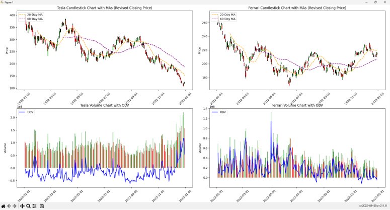
Draw a OBV indicator chart.
- OBV (On Balance Volume) indicator calculation formula
Today’s closing price < Previous day’s closing price → Today’s OBV = Previous day’s OBV - Today’s volume
Today’s closing price > Previous day’s closing price → Today’s OBV = Previous day’s OBV + Today’s volume
Today’s closing price = Previous day’s closing price → Today’s OBV = Previous day’s OBV
5.obv.py
import pandas as pd
import matplotlib.pyplot as plt
import matplotlib.dates as mdates

# Load Tesla and Ferrari stock data
tesla_data = pd.read_csv('tesla_quote.csv', parse_dates=True, index_col='Date')
ferrari_data = pd.read_csv('ferrari_quote.csv', parse_dates=True, index_col='Date')

# Define the period for both charts (e.g., '2022-01-01' to '2022-12-31')
start_date = '2022-01-01'
end_date = '2022-12-31'

# Filter dataframes to include only the specified period
tesla_data = tesla_data[(tesla_data.index >= start_date) & (tesla_data.index <= end_date)]
ferrari_data = ferrari_data[(ferrari_data.index >= start_date) & (ferrari_data.index <= end_date)]

# Create subplots with 2 rows and 2 columns to display charts side by side
fig, ((ax1, ax2), (ax3, ax4)) = plt.subplots(nrows=2, ncols=2, figsize=(18, 12))

# Define candlestick colors
up_color = 'g'
down_color = 'r'

# Plot Tesla candlesticks and 20-day moving average
for idx, row in tesla_data.iterrows():
    open_price = row['Open']
    close_price = row['Close']
    high_price = row['High']
    low_price = row['Low']

    if close_price > open_price:
        color = up_color
        rect_height = close_price - open_price
        y = open_price
    else:
        color = down_color
        rect_height = open_price - close_price
        y = close_price

    ax1.add_patch(plt.Rectangle((mdates.date2num(idx) - 0.2, y), 0.4, rect_height, fill=True, color=color, zorder=2))
    ax1.plot([mdates.date2num(idx), mdates.date2num(idx)], [low_price, high_price], color='black', zorder=1)

# Calculate 20-day moving average for Tesla based on revised closing price
tesla_data['20D_MA'] = tesla_data['Close'].rolling(window=20).mean()
ax1.plot(tesla_data.index, tesla_data['20D_MA'], label='20-Day MA', color='orange', linestyle='--')

# Calculate 60-day moving average for Tesla based on revised closing price
tesla_data['60D_MA'] = tesla_data['Close'].rolling(window=60).mean()
ax1.plot(tesla_data.index, tesla_data['60D_MA'], label='60-Day MA', color='purple', linestyle='--')

# Set x-axis format for Tesla chart
ax1.xaxis.set_major_formatter(mdates.DateFormatter("%Y-%m-%d"))
ax1.set_ylabel('Price')
ax1.set_title('Tesla Candlestick Chart with MAs (Revised Closing Price)')
ax1.tick_params(axis='x', rotation=45)
ax1.legend(loc='upper left')

# Plot Ferrari candlesticks and 20-day moving average
for idx, row in ferrari_data.iterrows():
    open_price = row['Open']
    close_price = row['Close']
    high_price = row['High']
    low_price = row['Low']

    if close_price > open_price:
        color = up_color
        rect_height = close_price - open_price
        y = open_price
    else:
        color = down_color
        rect_height = open_price - close_price
        y = close_price

    ax2.add_patch(plt.Rectangle((mdates.date2num(idx) - 0.2, y), 0.4, rect_height, fill=True, color=color, zorder=2))
    ax2.plot([mdates.date2num(idx), mdates.date2num(idx)], [low_price, high_price], color='black', zorder=1)

# Calculate 20-day moving average for Ferrari based on revised closing price
ferrari_data['20D_MA'] = ferrari_data['Close'].rolling(window=20).mean()
ax2.plot(ferrari_data.index, ferrari_data['20D_MA'], label='20-Day MA', color='orange', linestyle='--')

# Calculate 60-day moving average for Ferrari based on revised closing price
ferrari_data['60D_MA'] = ferrari_data['Close'].rolling(window=60).mean()
ax2.plot(ferrari_data.index, ferrari_data['60D_MA'], label='60-Day MA', color='purple', linestyle='--')

# Set x-axis format for Ferrari chart
ax2.xaxis.set_major_formatter(mdates.DateFormatter("%Y-%m-%d"))
ax2.set_ylabel('Price')
ax2.set_title('Ferrari Candlestick Chart with MAs (Revised Closing Price)')
ax2.tick_params(axis='x', rotation=45)
ax2.legend(loc='upper left')

# Plot Tesla volume chart with color-coded bars for daily change and OBV
tesla_data['VolumeChange'] = tesla_data['Volume'].diff()
tesla_data['VolumeColor'] = tesla_data['VolumeChange'].apply(lambda x: 'g' if x >= 0 else 'r')
ax3.bar(tesla_data.index, tesla_data['Volume'], color=tesla_data['VolumeColor'], alpha=0.7)
ax3.set_ylabel('Volume')
ax3.set_title('Tesla Volume Chart with OBV')
ax3.xaxis.set_major_formatter(mdates.DateFormatter("%Y-%m-%d"))
ax3.tick_params(axis='x', rotation=45)

# Calculate OBV for Tesla
tesla_data['OBV'] = tesla_data['VolumeChange'].cumsum()
ax3.plot(tesla_data.index, tesla_data['OBV'], label='OBV', color='blue')
ax3.legend(loc='upper left')

# Plot Ferrari volume chart with color-coded bars for daily change and OBV
ferrari_data['VolumeChange'] = ferrari_data['Volume'].diff()
ferrari_data['VolumeColor'] = ferrari_data['VolumeChange'].apply(lambda x: 'g' if x >= 0 else 'r')
ax4.bar(ferrari_data.index, ferrari_data['Volume'], color=ferrari_data['VolumeColor'], alpha=0.7)
ax4.set_ylabel('Volume')
ax4.set_title('Ferrari Volume Chart with OBV')
ax4.xaxis.set_major_formatter(mdates.DateFormatter("%Y-%m-%d"))
ax4.tick_params(axis='x', rotation=45)

# Calculate OBV for Ferrari
ferrari_data['OBV'] = ferrari_data['VolumeChange'].cumsum()
ax4.plot(ferrari_data.index, ferrari_data['OBV'], label='OBV', color='blue')
ax4.legend(loc='upper left')

# Adjust layout and show all charts
plt.tight_layout()
plt.show()